Abstract

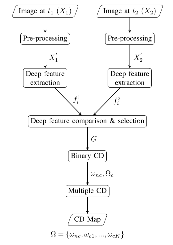
The DCVA(Deep Change Vector Analysis) is change detection methology that based on vector analysis of 'Deep feature extraction' and 'feature comparison'. This model consists of 2 parts. ('Deep feature extraction' and 'feature comparison')

At first, Bi-temporal image pair get through to pretrained ResNet, which for remote sensing image's semantic segmentation. then feature maps of image pair is extracted from the certain layers of ResNet. (Deep feature extraction)

The Feature comparison module compares the creatred 2 feature maps and selects changed vector between of them. The changed vector is represented to binary Change Detection maps.

Summary

Input

Image X1, X2 that have 1024 X 1024 X 4 (RGB+NIR) Those two images must be taken in same sensor.

Preprocessing

The input bitemporal image X1, X2 should be preprocessed for removing distortions.

(1) invert image to obtain radiance value and radiometrci normalization.

(2) orthorectification (정사보정)

(3) Pansharpening (팬샤프닝, 업샘플링)

(4) coregistration

The orthorectification, pansharpening is applied to multispectral bands. However, coregistration is applied to panchromatic band, beacause panchromatic bands' resolution is 4 times higher than multispectral bands.

The pansharpening is applied by Gram-Schmidt method. This preprocessing step mitigate the error that caused by radiometric elements, misalignments, atmosphere.

Deep feature extraction

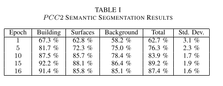
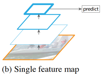
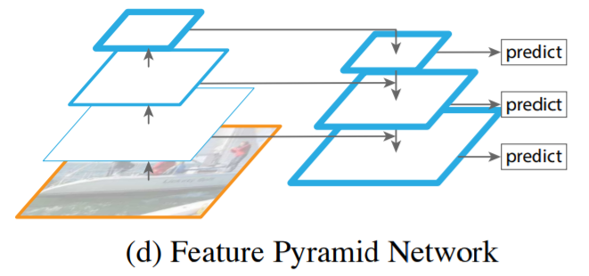
The preprocessed image pair (X1', X2') separately input to pretrained ResNet Model and the features extracted from certain layers of ResNet. In this paper, Volpi and Tuia is used to pretrained ResNet Model. This model consists of 23 ResNet layers. The 2, 3, 5, 8, 10, 11, 23 layers is used for extraction. Each layers create their own feature map and perform 'Deep feature comaprison' separatly.

Deep feature comparison & selection

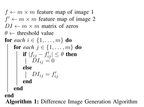
The feature map that finished deep feature extraction is subtracted to make difference vector. ( f2i - f1i )

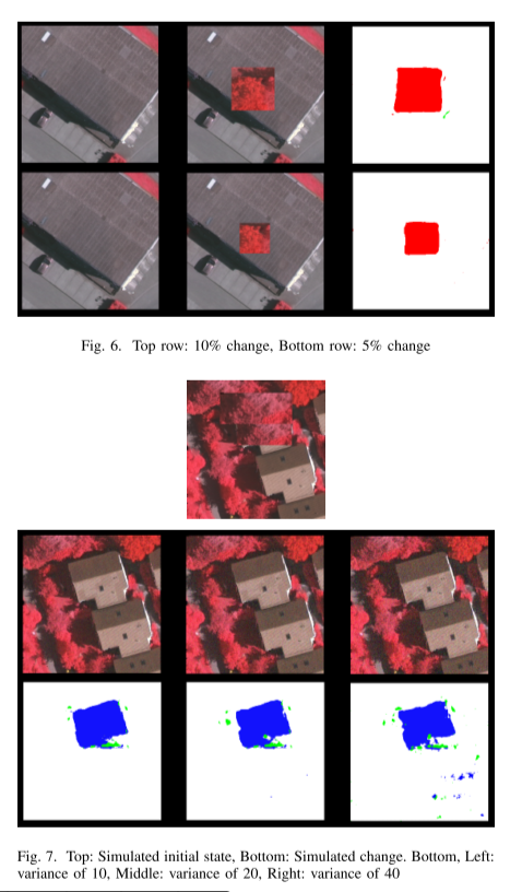
The difference vector is divided spatially to 4 patches. Then variance of vector is computed for each patch.

If the variance become higher, probability of change increases. So we sort all of feature indices by variance in descending order and select certain percentage of feature indices.

This sortation and selection performs in each patch, thus we concatenate all selected feature maps from 4 patches. This result feature map of this selection is called 'deep change hyper vector' or G vector

Change Detection

Compute deep magnitude 'rho'. (r, c is x cord, y cord)

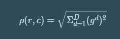
This 'rho' mapped to 1-dimension. By this mapping task, the D-dimension G vector is transformed to 1-dimension and main properties of change can be preserved. We convert 'rho' to 0 or 1 by otsu-threshold.

The '1' represents 'changed vector' and '0' is for 'unchanged vector'. Thus binary change map created.

Result

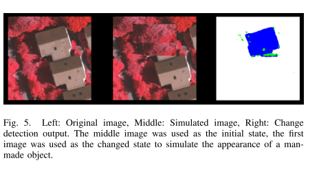
image 1

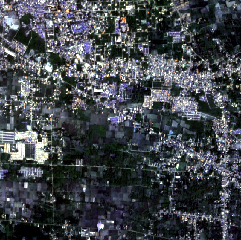
image 2

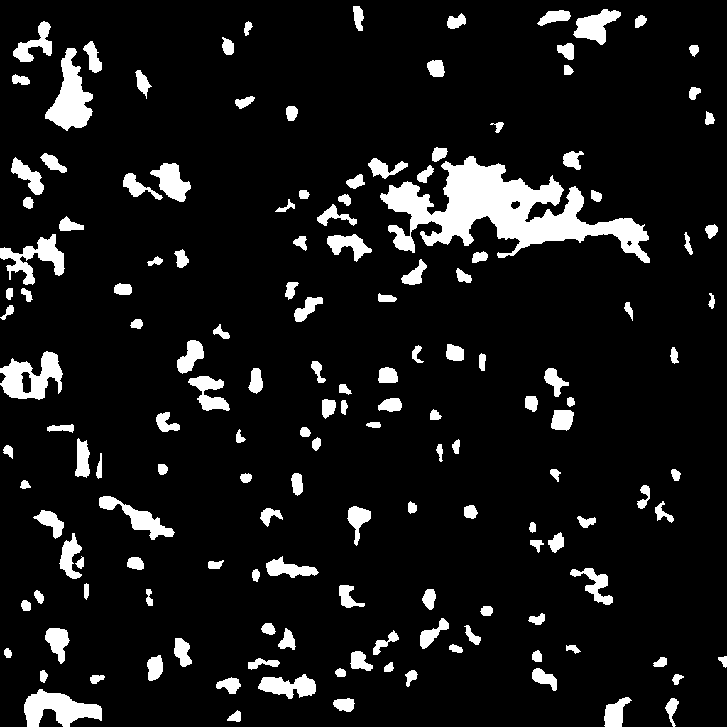
result

Submission result (2021-03-19)

In earthVison21 competetion, The 1st place of Binary change detection!

Summary

Current change detection

(1) Utilising either post-classification anlysis ⇒ classify contents of two different image, then compare them to identify difference.

(2) difference image analysis ⇒ constructs DI(difference image)

DI : highlight the differences between two same but temporally difference scene. In this paper, We will use (2) difference image analysis.

Main object

(1) determine the efficacy of using the feature maps generated by U-net of two images to create an effective DI (효과적인 DI 생성에 사용할 피쳐맵의 효능을 결정함)

(2) Accurately classify the changed part automatically

(3) Build a robust model from noise

(4) Build a image that represent detected changes using semantic segmentation

Model

Proposed model is based on U-net. It has two phases : (1) training (2) inference

(1) Training Phase

Dataset : Vaihingen dataset Total 33 satellite image from 1 larger TOP image.

Only 16 images have their corresponding ground truth set.

All images are 320 X 320 X 3.

All image pixel values for each color channel were nomalized (mean : 0.5, deviation 0.5)

Semantic segmentation

Training set : 15 images and their corresponding ground truth images.

Validation set : 1 image and its corresponding ground truth image.

Class : 3 semantic classes / buildings, immutable surfaces(kinds of roads and parking lots), backgroud (non of the other classes, like vegetation )

Change Detection

Since there's no temporally different images of same area, changes were simulated by editting manually.

20 random images were selected and each images has different changed-pixel rate (5, 10, 15%)

Training set : 20 images and their corresponding changed image by manually editting Class : None / Unsupervised

Training Parameter

Optimizer : Adam batch size : 4 loss function : log loss (cross-entropy function)

Measures of Accuracy

(1) Accuracy equation for predicting changed or unchanged (PCC1)

TP : Number of pixels that correctly classified as chaged

TN : Number of pixels that correctly classified as unchaged

FP : Number of pixels that incorrectly classified as chaged

FN : Number of pixels that incorrectly classified as unchaged

(2) Accuracy equation for predicting correctly classified (PCC2)

CC : Number of pixels that correctly classified as semantic class

IN : Number of pixels that incorrectly classified as semantic class

(2) Inference Phase

Modifing model to accept two images.

• Each feature maps from U-net's 5 levels are saved for the first image.
• • DI genereation Algoritm
    Compare first and second image's corresponding element pair.
    If absolute difference falls between 0 and a threshold, corresponding DI element becomes 0.
    Otherwise, DI element is generated by second image's feature map activation.When second image is accepted, DI is created at each 5 levels, using first and second images' feature map.

• Then, 5 DI images are used by the decoder in copy and concatenate, Insted of the feature maps generated by the second image encoding phase.
• Thus, the output of the model is semantically segmanted.

(3) About DI threshold

According to empirical test, threshold must differ at each U-net levels.

• Level 1 : 0.4
• Level 2 : 0.6
• Level 3 : 0.8
• Level 4 : 1.0
• Level 5 : 1.2

Model Hyperparameter

(1) Layer activation function : leaky ReLU (slop : -0.2) / Output layer : softmax

(2) Input size : 320 X 320 X 3 (RGB)

(3) Convolution operation : 1 stride 3X3, padding 1 / batch normalisation

(4) Deconvolution operation : 2 stride 3X3, padding 0 / batch normalisation

(5) Unet Encoder : Consist of 4 levels, 2 convolution ops and max pooling (2 stride 3X3 padding0)

(6) Unet bridge : 1 level, 2 convolution ops, no max pooling.

(7) Unet Decoder : Consist of 4 levels, 2 convolution ops and 1 Deconvolution ops

(8) Final level : 3 convolution ops

(9) Number of kernels : First level at 64, no changed in same level (Due to 1 padding), doubled at each encoding levels, reaching a total 1024 at bridge. Then halved at each decoding levels, reaching 64 at last level. Final convolution ops reduced channels to 3.

Result : Change Detection

Best performance served at epoch 15.

The model can detect difference of building's appearance, disregarding irrelevant pixels. Some small cluster of pixels appeared. This clusters depended on DI threshold values. (See DI threshold.)

Greater differences between 2 images makes grater differences in feature maps. Namely, 10% changed output was less accurate than 5% change output.

Gaussian noise was added to test robustness of the model. Low and moderate noise caused decrease of change classification accuracy. And if noise beacome larger, more decrease of accuracy appeared.

The model performed worst when changes are situated on the edge of an image. This is likely a result of kernel convolviong over fewer data points. This can be improved by cutting High-dimensional satellite images into overlapping subsets, or combining change detection signals generated by the overlapping areas.

Abstract

2019년 현재까지 Object Detection 분야 성능이 비약적으로 발전했다. 이를 넘어 Google에서 성능을 비약적으로 향상시킨 EfficientDet을 개발했다.

EfficientDet은 EfficientNet을 Backbone으로 하는 Bi-FPN(Bi-Feature Pyramid Network)을 특징추출 네트워크로 사용했다. 기존 FPN에서 사용했던 feature fusion을 폐기하고 Weighted Feature Fusion을 새로 고안해 적용했다.

그 결과 2019년 11월 기준 SOTA 성능을 보이고 있다.

Summary

Bi-FPN을 설명하기 앞서 FPN의 기본 구조를 알아야 한다.

최초 CNN은 입력 이미지를 Conv 레이어에 입력시켜가며 다중 해상도 피쳐맵을 만들어냈다.

하지만 아웃풋으로 사용하는 것은 가장 저해상도의 피쳐맵이었다. 이를 Single feature map이라 한다.

가장 마지막 압축 특징을 사용하기 때문에 성능이 떨어졌다.

이때 아웃풋으로 사용되지 않는 각 Conv 단계의 피쳐맵들을 모두 아웃풋으로 Predict 하려는 시도가 생겼다.

각 단계에서 독립적으로 피처맵을 추출해서 객체를 탐지한다. 이를 Pyramidal Feature Hierachy라 한다.

하지만 이는 각 레벨 간 정보교환이 없이 독립된 특징만 도출한다는 단점이 있다.

상기한 단점을 가진 PFH를 보완하고자 각 단계 별 추출된 피쳐 맵 간 정보를 교환시켜 고해상도 피쳐맵을 도출하는 시도가 생겨났다.

가장 저해상도인 피쳐맵을 2배로 Up sampling 시켜 크기를 4배 키우고, 대칭 대응쌍인 Down sampling 과정의 동일크기 피쳐맵과 Element-wise addition으로 병합시킨다.

이는 U-Net의 과정과 비슷하다. (Skip connection)

본 논문 작성자인 Google 연구팀은 기존 FPN에서의 Upscailing 과정만 사용하고, Skip connection 과정에서 피쳐 맵 간 병합(Feature Fusion)이 단순한 Element Wise Addition으로 이뤄진다는 점에 집중했다.

연구팀은 기본 FPN에서 Up scailing 실행 후 다시 Down scailing을 실행하는 PANet과, 동일 scale이 아닌 다른 scale 간 connection도 존재하는 (Cross scale connection) NAS-FPN을 제안했다.

여기에 PANet의 구조를 기반으로 NAS-FPN의 Cross scale connection을 사용한 Simplified PANet을 고안했고,

최종적으로 Simplified PANet에서 동일 단계 간 shortcut을 설정해 더 많은 feature를 fusion할 수 있게 한 Bi-FPN을 완성했다.

각 Connection에 사용되는 Feature Fusion은 단순한 Elementwise-Addition(크기가 같은 행렬 간 연산에서 요소들만 더하거나 곱함)을 사용하기 때문에 input feature들 간 중요도가 모두 무시된다는 단점이 있다. (Conventional FF)

이를 해결하기 위해 가중치를 부여한 Weighted Feature Fusion을 고안했다.

가중치는 scalar, vector, multi dimensional tensor 모두 사용 가능한데, 본 논문에선 scalar가 실험결과 제일 우월해서 이를 사용했다. scalar 형식인 가중치를 단순히 곱해서 더하면 (Unbounded FF) 학습 불안정성을 유발할 수있다.

따라서 Softmax을 사용해 0~1 사이 값으로 정규화했다. (Softmax FF)

하지만 Softmax 특성상 분모에 0이 들어가 계산과정에 오류가 날 가능성이 약간이나마 존재한다.

물론 값이 Relu를 거치므로 0이 되진 않지만 안전장치가 있으면 나쁠 건 없다.

이를 보완코자 0.0001크기의 입실론을 설정해 분모에 더해줬다. 그 결과 Fast normalized Feature Fusion 식이 탄생했다.

상기한 BiFPN과 Fast normalized FF를 모두 적용한 EfficientDet 구조는 다음과 같다.

ImageNet으로 Pretrained 된 EfficientDet을 백본으로, 최종 output부터 직전 5개 단계의 Feature map들을 BiFPN 형식으로 Feature Fusion을 진행했다. 그리고 그 아웃풋을 Box prediction과 Object Classification부로 따로 나눈 Conv 레이어에 입력해 다시 Feature map을 그렸다.

EfficientDet은 B0부터 B6를 사용했다. Compound scailing은 다음과 같은 표로 설정했다.

성능은 다음과 같았다.

보다시피 mAP와 파라미터 수, FLOPS, CPU-GPU Latency가 월등히 낮은 것을 볼 수 있다.

이는 2019년 11월 기준 SOTA에 해당한다.

Abstract

기존 CNN에서 Width (Convolution 채널의 개수, 3x3 Conv을 몇개를 사용할 것인가), depth (레이어의 개수), resolution (해상도)를 최적 상태로 변경한다면 압도적으로 성능이 좋아진다. 3가지 변수들을 최적 상태로 만들기 위해 Compound Scaling을 제안한다.

Summary

변인 통제를 위해 모델을 고정하고 depth, width, resolution 3가지를 조절해야 하는데, 모델은 AutoML을 통해 모델을 탐색했다. 이를 EfficientNet-B0로 명명한다. B0 구조는 다음과 같다.

Compound Scailing : 아래 수식을 참조하자. 노란색으로 강조한 등식을 유지하며 알파 , 베타, 감마와 파이를 변경해준다. 이때 알파는 d를 2배 키울 때 FLOPS(GPU의 초당 부동소수점 연산량)도 2배 늘어나서 1제곱이지만, 베타와 감마는 각각 w와 r이 두배 늘어날 때 FLOPS가 제곱으로 늘어나 2제곱을 설정했다.

논문에서는 먼저 파이를 1로 설정 후 해당 등식을 만족하는 최적의 알파, 베타, 감마값을 찾았다. (알파 : 1.2, 베타 : 1.1, 감마 : 1.15) 그런 다음 파이를 정수배로 늘려가며 모델의 사이즈를 키웠다.

결과적으로 기존 CNN과 비슷한 정확도를 보이면서 parameter수와 FLOPS 수를 상당히 절약했다. 또 ImageNet 데이터셋에서 최고등급을 기록한 GPipe보다 정확도가 더 높았다. 결과표는 다음과 같다.